~ computer vision fun ~ with photogrammetry

A couple months ago we became interested in computer vision, a broad subject of teaching computers how to see.  We began by feeding images into Grasshopper, a visual scripting plug-in for Rhino, and generating printable 3D models. Photogrammetry opened up the possibility to generate models from a variety of sources, from things directly in front of you to videos found online.  There are a number of exciting practical and creative applications for photogrammetry.  While we played around with a variety of proprietary and open source programs, it seemed important to develop an accessible workflow of all open or shared source software for anyone to explore the multitude of possibilities.  While the software we used was amazing in many ways, they definitely have their flaws and limitations when compared to their proprietary competitors.

–Anna Brancaccio + Catie Buhler

Here are links to tutorials that we found most helpful:

VisualSFM –> Meshlab: Here

VisualSFM–>Meshlab–>Blender: here
 

VisualSFM to Meshlab

VisualSFM Overview VisualSFM is a free, shared-source photogrammetry program created by Changchang Wu. You can upload a series of jpg.,ppm. or pgm. images to VisualSFM to create a dense point cloud that can be turned into a textured mesh using Meshlab.

Tips for collecting images for vSFM In our experience VisualSFM has a much easier time constructing point clouds of specific objects, rather than spaces or more general landscapes; it seems to sort of average out all the matches it makes between images, and focus on creating a point cloud for only the densest area of matches rather than creating a general point cloud of everything that it recognizes.It has a hard time recognizing reflective or transparent materials. Just know that the types of images, and the variety amongst the images you select have a big influence on the resulting point cloud. I would recommend using images that were taken at relatively similar distances from your subject, close-ups or zoomed out images have a tendency to dilute the quality of the point cloud. It’s best to take photos as if you were lining up a grid, and also allow a lot of overlap between images, this will help matches be creating amongst the images, and will give you a more detailed point cloud.

Downloading vSFM — http://ccwu.me/vsfm/ We installed the 64-bit version for Windows. Their are installation guides for Windows, Linux, and Mac on the VisualSFM website which is listed above. To install for Windows, all we had to do was download VisualSFM from the installation guide (http://ccwu.me/vsfm/install.html), then install Yasutaka Furukawa’s CMVS software (for dense reconstruction), we used Pierre Moulon’s binaries, https://code.google.com/p/osm-bundler/downloads/detail?name=osm-bundler-pmvs2-cmvs-full-32-64.zip You must put the CMVS/PMVS binaries into your VisualSFM folder that was created when you downloaded the program, otherwise it will not work properly. The only issue we weren’t able to resolve, was that we never got our command line running, although a friend downloaded VisualSFM for Linux, and had no issue with the command line. Creating a dense point cloud

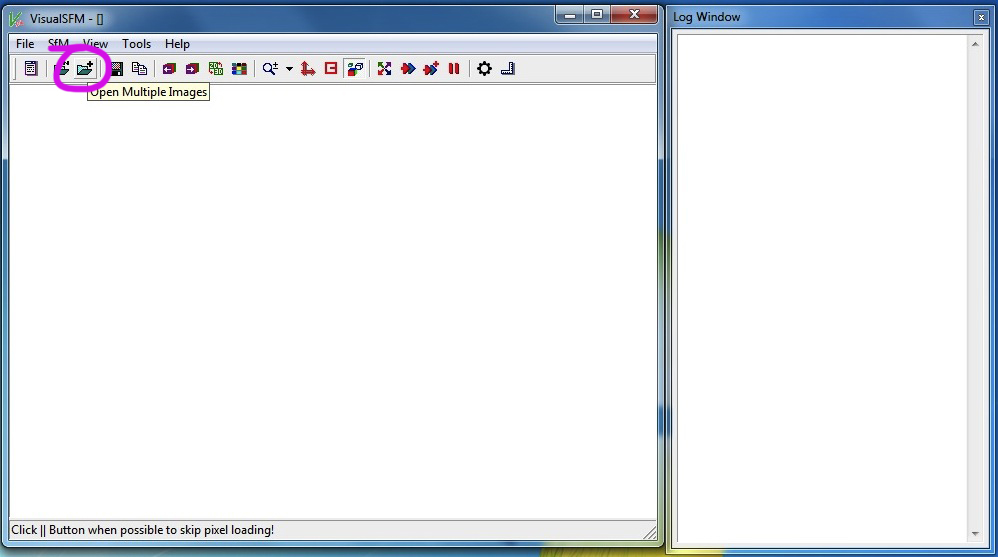
Open multiple images into VisualSFM by selecting the open-multi images icon.

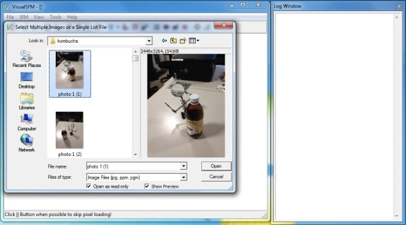
Select your images, it’s best to keep them all in their own folder, as VisualSFM creates extra files paired with each of the images when it matches them to each other.

Once all your images have uploaded, select the icon with the four arrows to begin the sifting process, VisualSFM will search for matches amongst the images, you can see this process in the log window.

When the matching has finished, the log window should say, “compute missing pairwise matching, finished”. Next you will create the sparse reconstruction, using the compute 3D construction icon.

Once the sparse reconstruction has been made the log window should say, “run full 3D construction, finished”. Then you can create the dense point cloud using the CMVS icon, this step will take the longest to compute.

You have to save out the folder that will be creating during the dense 3D construction inside your VisualSFM folder.

When the dense construction is finished, the log window should say, “run dense construction finished”. You can switch your view between the sparse reconstruction and the dense point cloud by using your tab key. Here you will see all the camera positions that have been detected. Once this step is finished you are ready to bring your dense point cloud into Meshlab to create your textured mesh!

 

 

MeshLab

Meshlab is free and open source software designed for editing unstructured meshes typically produced by 3D scans.  We will be using Meshlab to transform our point clouds into meshes as well as to quickly generate the UV textures for our meshes from the collection of photos used to make the point clouds. Meshlab is pretty intuitive, and the texture mapping works great.  However, we were having some problems with Meshlab crashing at various points in the process even with our smaller point clouds, so it’s a good idea to frequently export your current version of the file, especially since there is no undo option in Meshlab.  The second issue we had was trying to generate the poisson mesh using a point cloud file we had already edited. You can download Meshlab here for Mac OS X, Linux, and Windows. Mr. P Meshlab Tutorials is a great resource for learning how to use Meshlab.

Here we go…

First, go to File ->Open Project and navigate to the .nvm.cmvs folder generated by VisualSFM when constructing the point clouds.  That should bring you to another folder labeled 00.  In here you should find the bundle.rd.out file.  Select this.  Meshlab should automatically prompt you to select a text file.  Select list.txt.

This should import the sparse reconstruction into Meshlab along with the same camera positions created in VisualSFM. Then, go to Render -> Show Cameras.  If the toolbar on the right of the screen is hidden, click the layer icon.  You should see a list of layers (just one right now) and further to the bottom, a box labeled Show Cameras.  Change the scale from 5 to around .0001 or just keep adjusting the number until the cameras are visible.  Then hit save.

After this you can hide the sparse reconstruction by hitting the eye to the left of the layer.  You can also deselect Show Cameras by going back to the Render drop-down menu. Now that we’ve inserted the cameras, we can bring in the dense reconstruction by going to File -> Import Mesh and navigating to the Models folder within the nvm.cmvs folder.  Then choose the .ply file created in VisualSFM.  If the point cloud is huge, VisualSFM will export the point cloud in multiple .ply files.  We came across this with our first set of images of a gazebo in which VisualSFM exported three ply. files.  While they can all be taken into Meshlab and merged, we were unable to generate a UV texture for merged meshes.  Probably with a little more time using Meshlab we could figure out a solution to this problem in Meshlab.

As of right now, we have been using an additional free and open source software called Cloud Compare which is exclusively meant for editing point clouds and meshes and is frequently used in conjunction with Meshlab. In Cloud Compare we were able to easily merge the multiple ply files to form a single point cloud.  When we merged it this way, we were able to import the merged ply into Meshlab and generate a color and texture file. Steps on how to merge .ply files in Cloud Compare can be found at the end of the tutorial.

Once you import the ply file, which is your dense reconstruction, you can delete the sparse reconstruction layer if you want by right clicking the layer and selecting Delete Mesh Layer.  The sparse reconstruction is only needed for setting the camera positions in place, and once they are imported in correctly, they will stay there even after the sparse reconstruction layer has been deleted.  However, if you delete this layer before importing the ply, Meshlab will crash.  Meshlab is extremely useful in a lot of ways, but is also very finicky. Now you can go in and clean up the point cloud.

Select the point selection icon circled above in the tool bar.  From there you can group select sections of the point cloud that you want to get rid of before you generate the poisson mesh.  Clearing floating or misplaced points with help to generate a cleaner, more accurate mesh.

Select the delete selected vertices icon circled above in the tool bar to clear the points you want to remove.

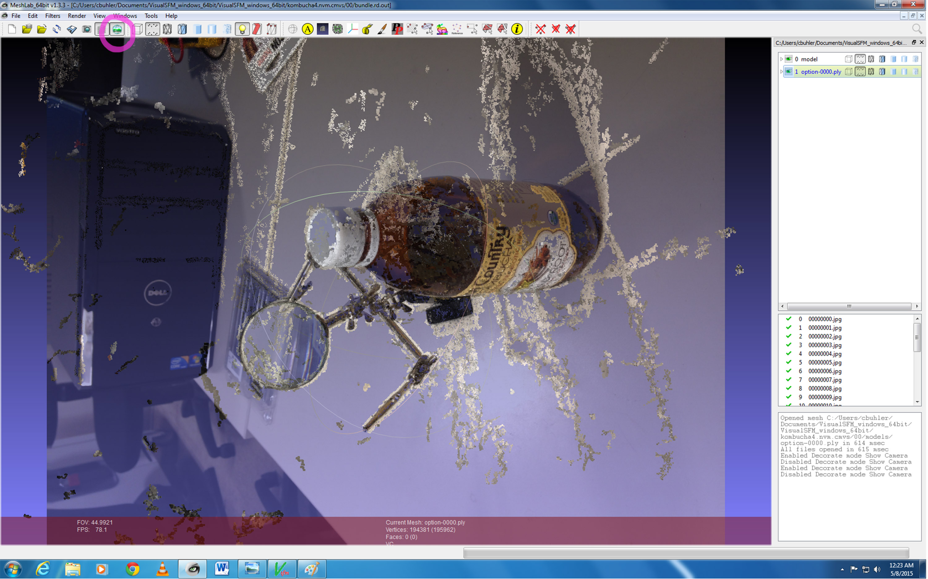
Select the Show Current Raster Mode icon circled above to check if the camera positions are correctly aligned to the dense reconstruction.  I’ve never had to readjust the camera positions.  For the most part, the points and camera angles have been positioned perfectly.  The occasional problems with this step that we came across was  typically an issue with the files from VisualSFM, so if they look really off here, I would go back into VisualSFM and regenerate the point clouds. You can click the icon a second time to close this setting once it has been checked.

Now that you’ve cleaned up the point cloud and checked camera positions, you can generate the poisson mesh.  Go to Filters -> Point Set -> Surface reconstruction: Poisson.

Depending on the level of detail of your model, you probably want to increase the Octree Depth.  We found for most of our models we could go up to 12 before Meshlab would crash.  However, you may want to make a lower poly mesh depending on the models intended use.  We ran into trouble with some of our denser point clouds where we would make a really accurate, high poly mesh with the Octree depth at 12, but when imported into Blender, would slow our game play down.  One of the advantages of photogrammetric modeling is that you can use low poly meshes with a highly detailed UV texture and end up with a pretty accurate looking rendered model. We kept the rest of the settings around their default values, but it’s a good idea to experiment with the different settings side they depend on your particular model.  By increasing the Solver Divide, you can make the model a little lighter weight.  Increasing the Samples per Node you can smooth out your mesh if you want.

Here is my resulting poisson mesh with the Octree Depth set to 8.  I still have the ply layer visible which is where the color comes from.

You can now clean up your mesh if you want in a similar way as with your point cloud.  Select the Face Selection bottom to the right of the Point Selection button in the tool bar.  Then hit the the Delete Faces button to the right of the Delete Vertices button also in the tool bar at the top of the screen. Then, remove any non manifold edges in the mesh by going to Filters-> Selection-> Select non-manifold edges.  Then select the Delete Vertices icon we used before. Now we can start generating the color and texture files for the mesh.  Meshlab has a method for doing this automatically which is a huge time saver and is amazingly accurate.  There is no need to unwrap the model and create/apply the textures in photoshop or other image editing programs.

Go to Filters-> Texture-> Parameterization from registered rasters.

These default settings worked well for our models.  Select apply if your settings match the ones in the box above. Then go to Filters-> Texture-> Project active rasters color to current mesh, filing the texture.

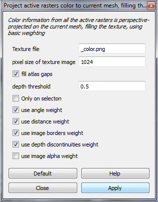
Change the file name of the color.  The default picture size worked fine for our models.  You can keep the same settings checked in the boxes, then hit apply.  This will save your color file for applying color to your mesh later on in other programs. The color should be projected onto the mesh. Then, to generate and apply your texture file to the mesh, go to Filters-> Texture-> Parameterization + texturing from registered rasters.

The same instructions for the color file apply to the texture.  Once you hit apply you should see the texture projected onto the mesh.

Finally, go to File-> Export Mesh as…  We export our models for as  Alias Wavefront Object or obj files for ease of use with Blender and Rhino.

Cloud Compare (if you need to merge multiple .ply files)

As noted above Cloud Compare is a free open-source program for editing point clouds and meshes, that is often used jointly with Meshlab. As of now we have really just used Cloud Compare to merge .plys. For every 50 cameras VisualSFM recognizes it usually creates a new .ply, so when dealing with a high quality point cloud you may end up with multiple .plys that need to be merged. We were having difficulty merging or even keeping the texture on our merged .plys in Meshlab, so instead we have been using Cloud Compare to merge the .plys that come out of VisualSFM, and then bringing them into Meshlab.

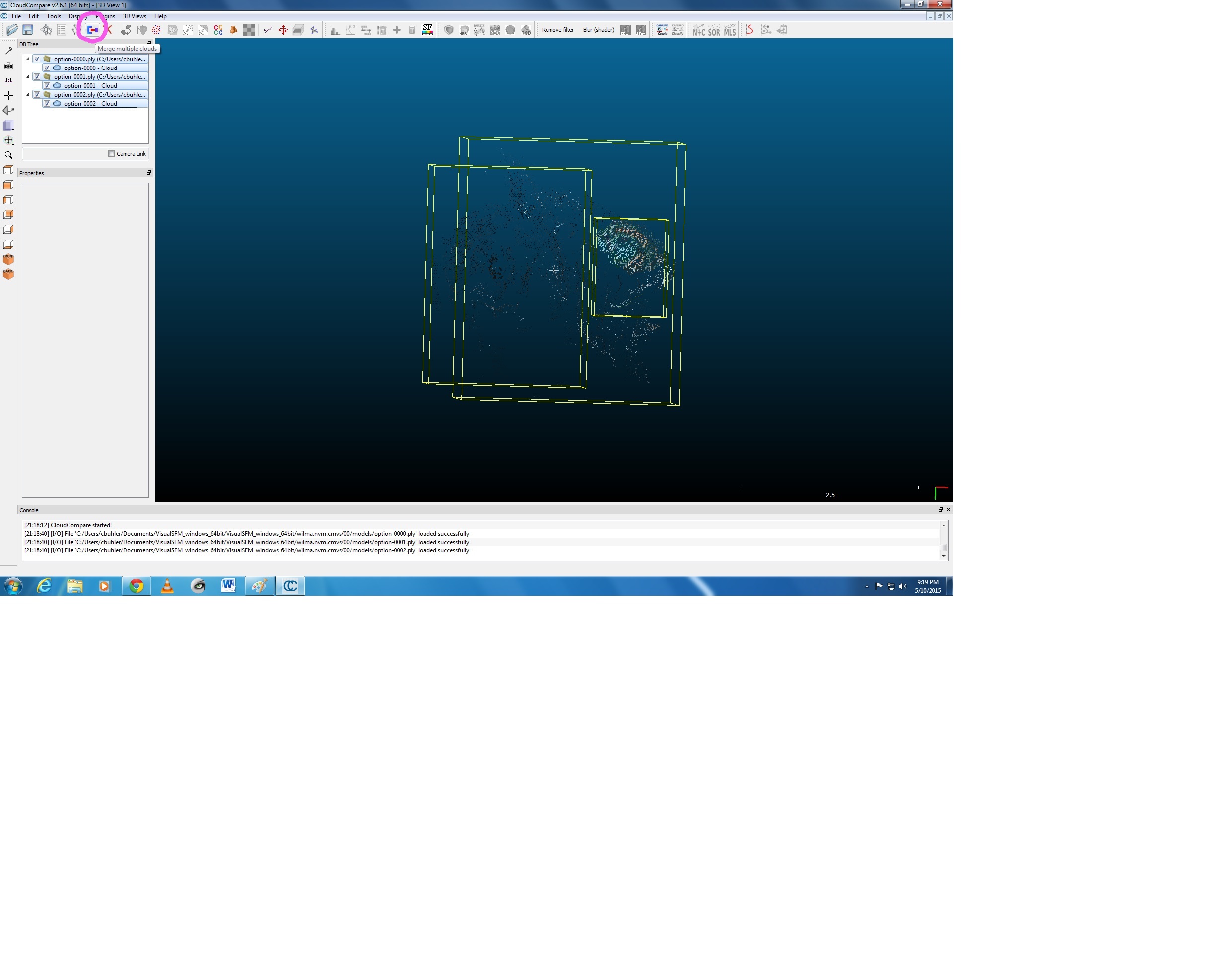
Begin by opening your multiple .plys at the same time into Cloud Compare, after you’ve hit open a window will come up, you can keep the default settings and just hit apply all 

Next select everything in your layers panel, and select the merge multiple clouds icon in the top left window

After you have merged the clouds you should see just one .ply and one cloud in your layers panel, your log window at the bottom may give you an error, ” (your file) is neither a cloud nor a mesh, can’t merge it!”, in my experience this error doesn’t actually prevent the .ply from merging.

After you have saved out your merged .plys in your models folder inside the nvm.cmvs folder you are working in, you can open the merged .ply in Meshlab and begin constructing your textured mesh!